Cuckoo Search and NatOptimToolbox
Cuckoo Search
The last days I was working on a fun side project: a toolbox with a collection of nature-inspired metaheuristic search algorithms. I published the toolbox called NatOptimToolbox here. It currently features six search algorithms:
- Artificial Bee Colony
- Cuckoo Search
- Bat Search
- Firefly Search
- Whale Optimization Algorithm
- Gray Wolf Optimizer
In this post I wanted to look a bit closer at the Cuckoo Search algorithm.

Source: wikimedia
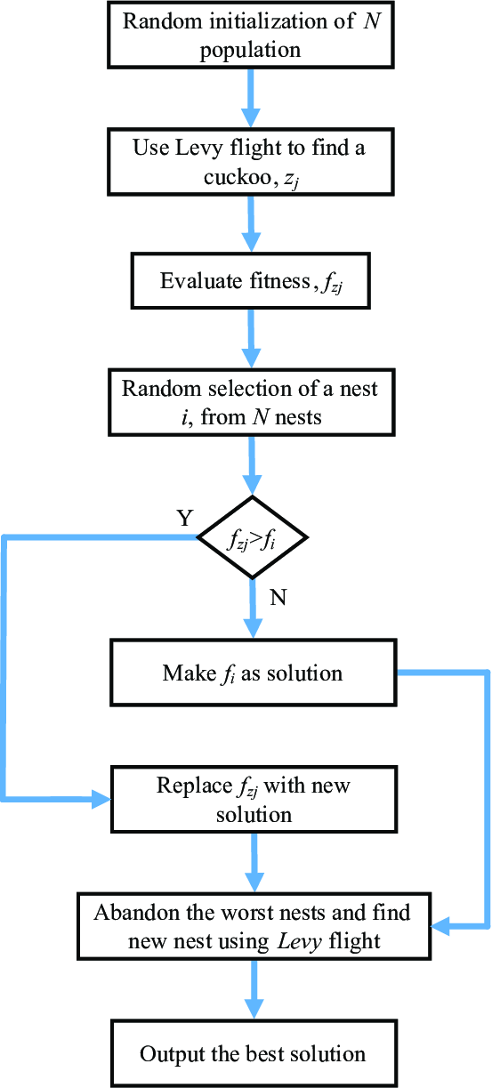
The Cuckoo Search algorithm is a metaheuristic search algorithm inspired by the brood parasitism of some cuckoo species. In these species, cuckoos lay their eggs in the nests of other host birds. If the host bird discovers the alien eggs, it may either throw them away or abandon its nest. The algorithm mimics this behavior to solve optimization problems.
-
Initialization: Generate an initial population of (n) host nests (solutions).
-
Get a Cuckoo: Randomly choose a cuckoo (solution) and generate a new solution using a Lévy flight process. This process is used because it allows the algorithm to perform local and global searches, simulating the unpredictable ways cuckoos lay eggs in various locations.
-
Evaluate and Choose Nests: Evaluate the fitness of the new solution. If the new fitness is better than the worst solution in the nest, replace the worst solution with the new solution.
-
Fraction (p_discovery): A fraction (p_discovery) of the worst nests are abandoned, and new ones are built. This introduces new solutions into the population, preventing premature convergence and encouraging exploration of the solution space.
-
Repeat: Repeat steps 2-4 until a termination condition is met (e.g., a maximum number of generations or an error tolerance).
-
Post-Process: The best solution found during the iterations is considered as the optimal solution to the problem.
I want to quickly demonstrate how to find the minimum for the Rosenbrock function, which is defined as:
np.sum(100 * (x[1:] - x[:-1]**2)**2 + (x[:-1] - 1)**2)
In case of a x having two elements the global minimum of the function will be [1, 1].
We will use the cuckoo search and the Nat[ure] Optim[ization] Toolbox.
I recommend setting up a virtual environment (make setup) first. Afterwards we install the requirements (make install). If you want to run an example or the tests you can use make run and make test respectively.
We first import the Population class, the CuckooSearch class and the Rosenbrock example function.
As for most metaheuristic algorithms we have to define the number of individuals in the population, how many attributes an individual has and the lower and upper bounds for the algorithm. Furthermore, we want to set a error tolerance for the optimization algorithm to stop and an upper limit of generations for optimization.
from population import Population
from optimizers import CuckooSearch
from example_functions import rosenbrock

population_size = 25
dim_individual = 2
lb = -5.12
ub = 5.12

error_tol = 0.01
n_generations = 100

objective_function = rosenbrock
As mentioned above we need two parameters for the cuckoo search algorithm: the probability for discovery and the lambda value for the levy flight.
Afterwards we can create our population and instantiate our CuckooSearch. Running it will reliable converge for this simple objective function.
p_discovery = 0.25
lambda_levy = 1.5

# Generate a population
population = Population(population_size,
                        dim_individual,
                        lb,
                        ub,
                        objective_function
                        )

cs = CuckooSearch(population,
                            limit,
                            n_generations,
                            error_tol=error_tol,
                            verbose=False
                            )
result = cs.run()
print("Cuckoo Search")
print(f"Best solution: {result.best_solution}")
print(f"Best solution fitness: {result.best_fitness:.2f}")
Output:
Best solution: [1.00078649 1.00156942]
Best solution fitness: 0.00
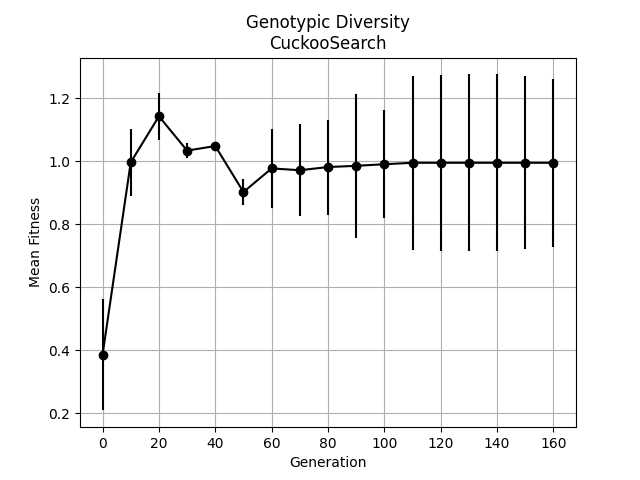
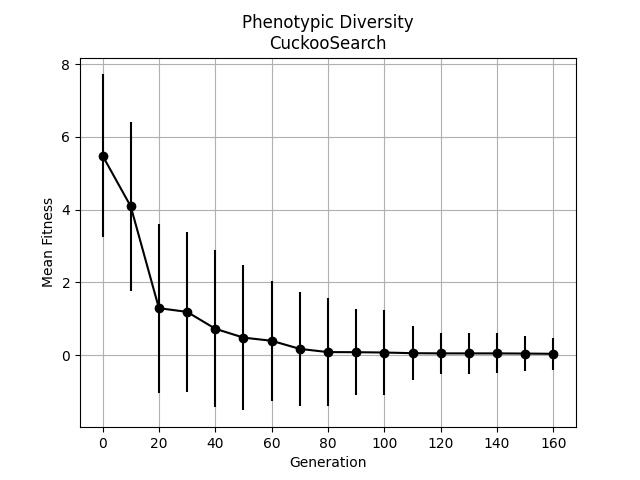
Finally we lock at some stats that we logged over the course of the optimization. We plot the phenotypic and genotypic diversity.
result.plot_phenotypic_diversity()
result.plot_genotypic_diversity()
In the genotypic diversity plot we can see how the traits of the individuals converge to one, which is the optimal solution for our spheric function.

Genotypic diversity
In the plot for the phenotypic diversity we see how the fitness of the value of the objective function decreases and lowers towards zero.

Phenotypic diversity
